> Machine Vision Defect Detection: A Complete Beginner's Guide
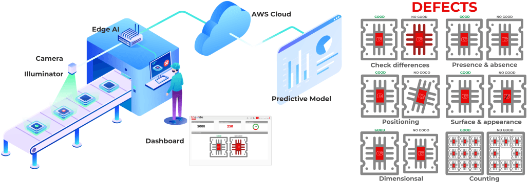
How AI-powered cameras find flaws in manufactured parts, from raw pixels to production line decisions. No engineering background required
This topic was inspired by a recent conversation I had with some experts in this field. During that conversation, I noticed how much I still had to learn about industrial AI vision. So I did some research and I'm here to share what I found.
What you'll learn
- What machine vision is and why factories use it.
- How industrial cameras and lighting work.
- How CNNs and Vision Transformers learn to detect defects.
- The full 5-stage inference pipeline.
- Common defect types and how each is detected.
- How to train your own model step by step.
- Key metrics, real case study, and costs.
1. Why Machines Inspect Better Than Humans (at Scale)
Picture a car brake component rolling off a production line at 600 parts per hour. Each one gets welded at 12 points. Every weld needs to be crack free, properly fused, and within 0.2 mm of spec. The old approach, one human inspector checks every 20th part under a magnifying glass.
That means 19 out of 20 parts shipped uninspected. A missed crack in a brake component doesn't just cost a warranty claim, it ends up in an accident report.
Machine vision closes that gap. And in the last five years, AI has made it accurate enough to trust on safety critical parts.
2. What Is Machine Vision?
Machine vision is the use of cameras and software to automatically inspect, measure, or identify objects on a production line.
A traditional machine vision system uses hand-coded rules "flag any pixel below brightness threshold X" or "reject if diameter < 48 mm." These work for simple defects but break the moment conditions change.
An AI-powered machine vision system uses a neural network trained on real images. Instead of rules, it learns patterns from examples. Show it 5,000 images of good welds and 500 of cracked welds, and it builds an internal model of what "defective" looks like, including subtle variations a rule based system would miss entirely.
3. Cameras and Lighting: The Foundation
Before any AI runs, you need a clean, consistent image. Most failed deployments stumble here not the model, but the optics and lighting setup.
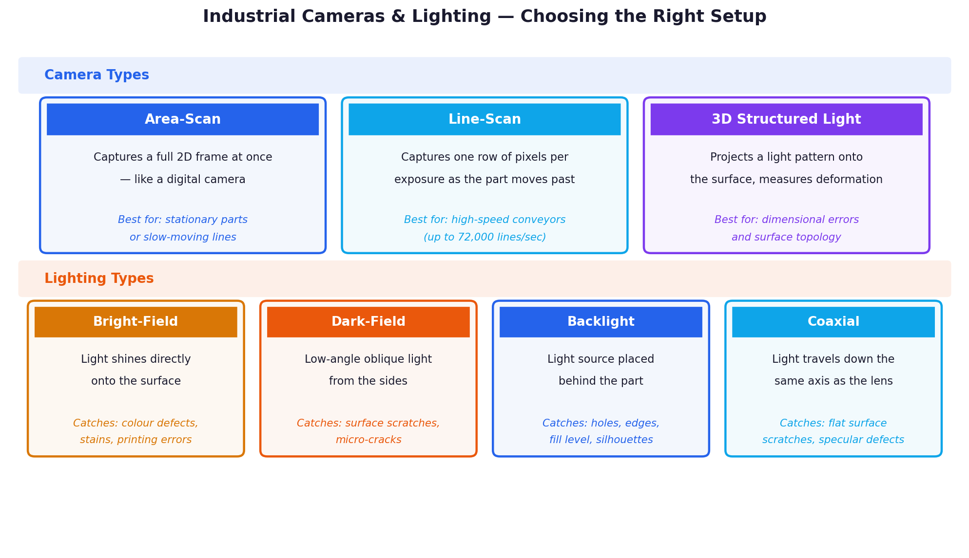
Key takeaway on lighting: A scratch invisible under direct overhead light becomes stark under low-angle raking light. A micro-crack in metal shows clearly under dark-field illumination. Lighting choice determines what defects are physically detectable at all — it is not cosmetic.
4. The Full Detection Pipeline
Once an image is captured, it moves through five stages. Each one has specific failure modes.
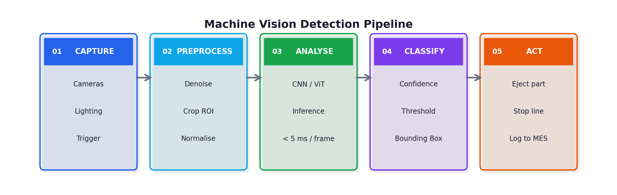
| Stage | What happens | Common failure mode |
|---|---|---|
| Capture | Camera photographs each part | Motion blur, inconsistent lighting |
| Preprocess | Denoise, crop, normalise | Over-aggressive cropping cuts defect region |
| Analyse | CNN / ViT runs inference (< 5 ms) | Wrong model architecture for defect type |
| Classify | Confidence score → pass/fail decision | Threshold set too tight or too loose |
| Act | Eject, log, alert | PLC integration lag, missed rejection window |
5. How CNNs Actually See Defects
The AI at the heart of most vision systems is a Convolutional Neural Network (CNN). Here is what happens layer by layer.
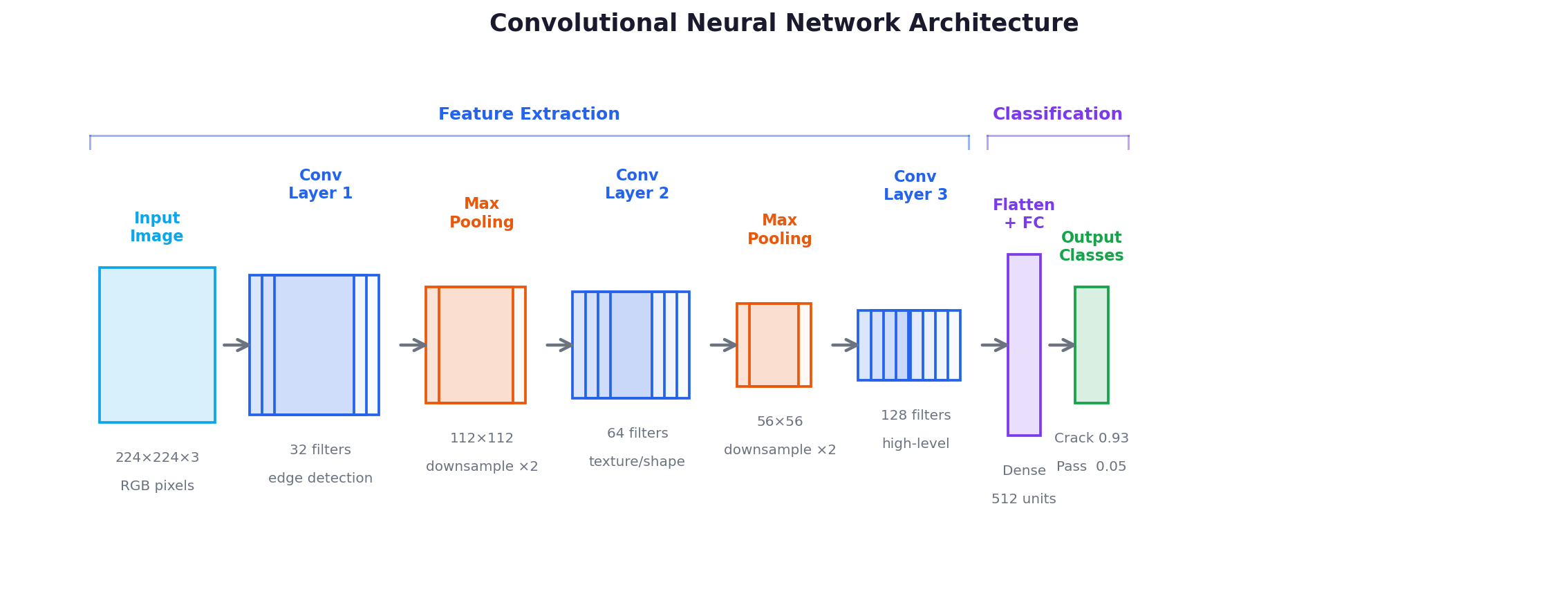
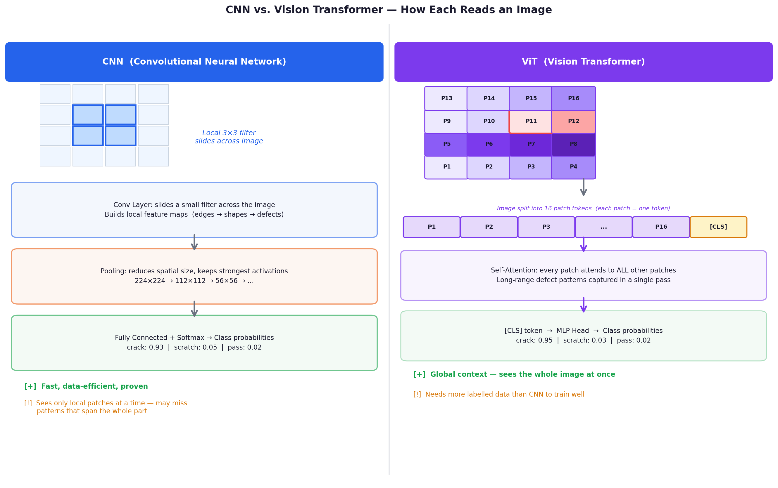
The network processes the image through a stack of layers. Early layers detect simple patterns (edges, gradients). Middle layers combine those into shapes and textures. Final layers produce class probabilities crack: 0.93, scratch: 0.05, pass: 0.02.
The network's knowledge lives in millions of numerical weights adjusted during training. Backpropagation computes how each weight contributed to a wrong prediction, and gradient descent nudges them in the right direction, repeated thousands of times over your dataset.
Transfer Learning: The Practical Key
Training a CNN from scratch needs millions of images. Transfer learning sidesteps this: start with a model pre-trained on ImageNet (1.2 million general images), then fine-tune its final layers on your defect data. This cuts requirements from millions of images to hundreds or a few thousand, making custom deployment practical for any factory.
| Model | Parameters | Best For |
|---|---|---|
| EfficientNet-B0 | 5.3M | First experiments, limited GPU |
| ResNet-50 | 25M | Balanced accuracy/speed |
| YOLOv8-m | 25M | Object detection + localisation |
| EfficientDet-D3 | 12M | Multi-defect detection |
6. Vision Transformers — The Next Step
CNNs dominated computer vision for a decade. Since 2020, Vision Transformers (ViT) have matched or exceeded CNN accuracy on many tasks, including defect detection.
The Core Difference
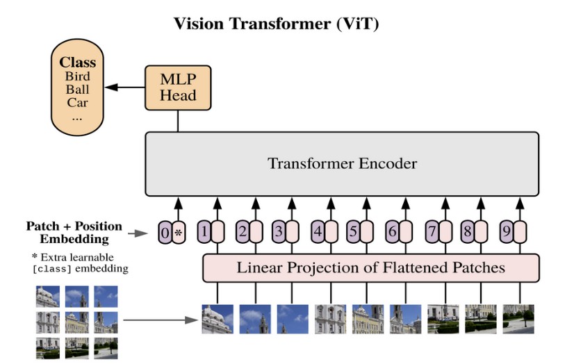
A CNN processes images through local convolutional filters, each filter only sees a small patch at a time. A Vision Transformer splits the image into fixed-size patches (e.g. 16×16 pixels), treats each patch as a token, and applies self-attention to model relationships between all patches simultaneously.
Why Global Context Matters for Defects
Some defects are not localised, they span the part, or their severity depends on where they sit relative to other features. A CNN building features patch-by-patch may miss a pattern that only becomes clear when the whole surface is considered at once. ViT's self-attention naturally models these long-range dependencies.
ViT Models for Industrial Inspection
| Model | Notes |
|---|---|
| ViT-B/16 | Original Vision Transformer, strong accuracy, needs ~1000+ images |
| DeiT-Small | Data-Efficient ViT — designed for smaller datasets, good for manufacturing |
| Swin Transformer | Hierarchical ViT, combines local + global attention, state-of-the-art on many industrial benchmarks |
| EfficientViT | Lightweight ViT for edge deployment |
Beginner note: You do not need to choose at the start. Train both CNN and ViT on the same data, compare validation recall, and keep the better one. In PyTorch with the
timmlibrary, swapping backbones is a 2-line change.
7. Common Defect Types
Different defects require different camera setups and model strategies.
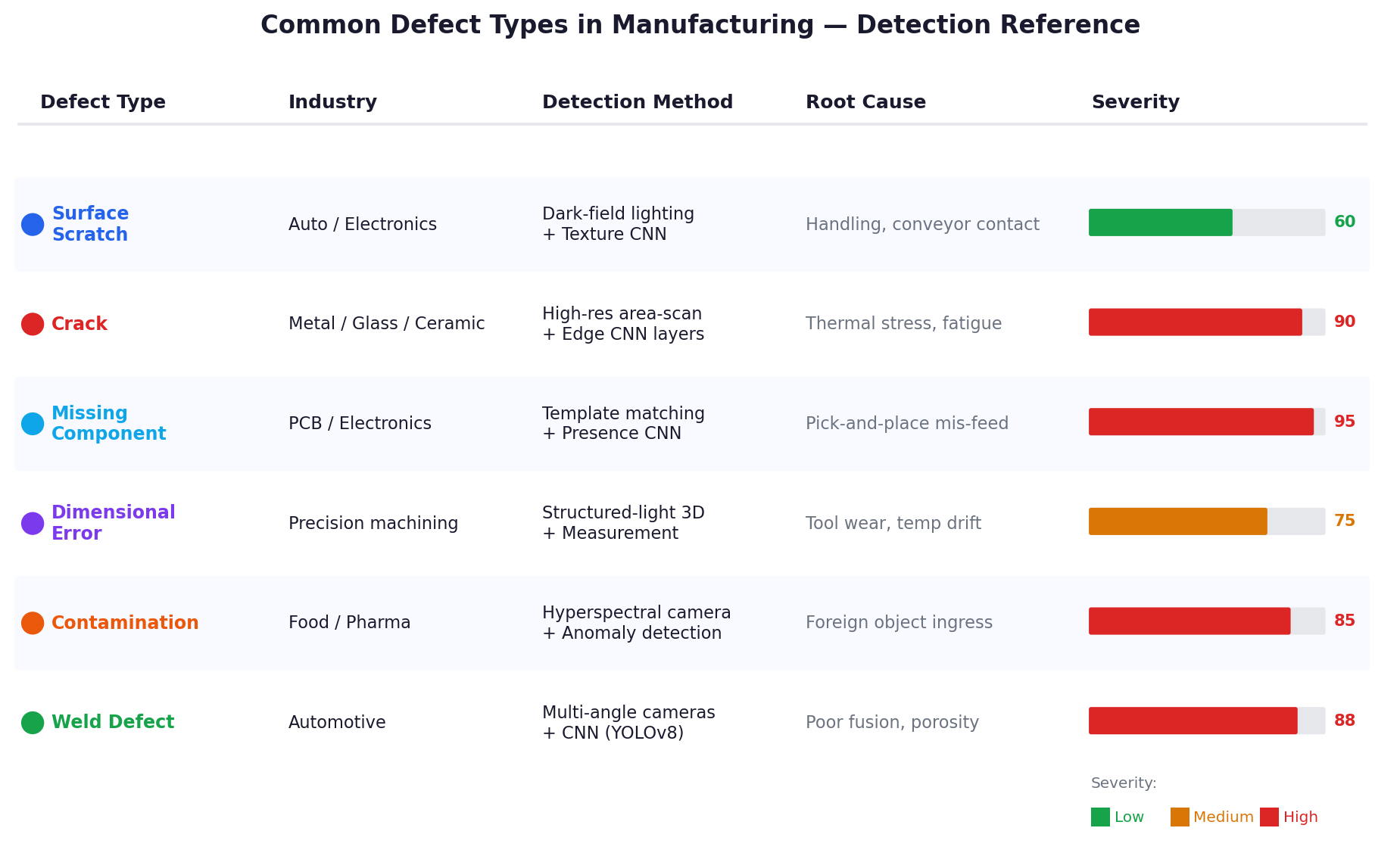
Reading the severity bar: Red (85+) means a missed defect has major downstream consequences safety risk, costly rework, or regulatory failure. Design your model threshold around the highest-severity defects on your line first.
8. AI Vision vs. Traditional Inspection
There are three main approaches to production inspection. Understanding the tradeoffs helps you pick the right one.
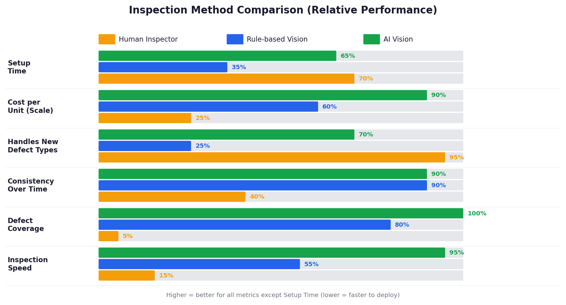
The shift from rule-based to AI vision is not about replacing good engineering with magic. It's about handling cases where writing rules becomes intractable, subtle surface textures, multi-class problems, or defect appearances that vary across batches and suppliers.
9. How to Train a Defect Detection Model
Training a custom model is not reserved for AI researchers. A small engineering team with a week of labelling effort can produce a production-ready model for most single-defect problems.
"You can follow this entire workflow in the companion GitHub project, it trains a ResNet-50 defect classifier from scratch, handles class imbalance, and evaluates with confusion matrix + F1: Defect Detection System for Manufacturing"
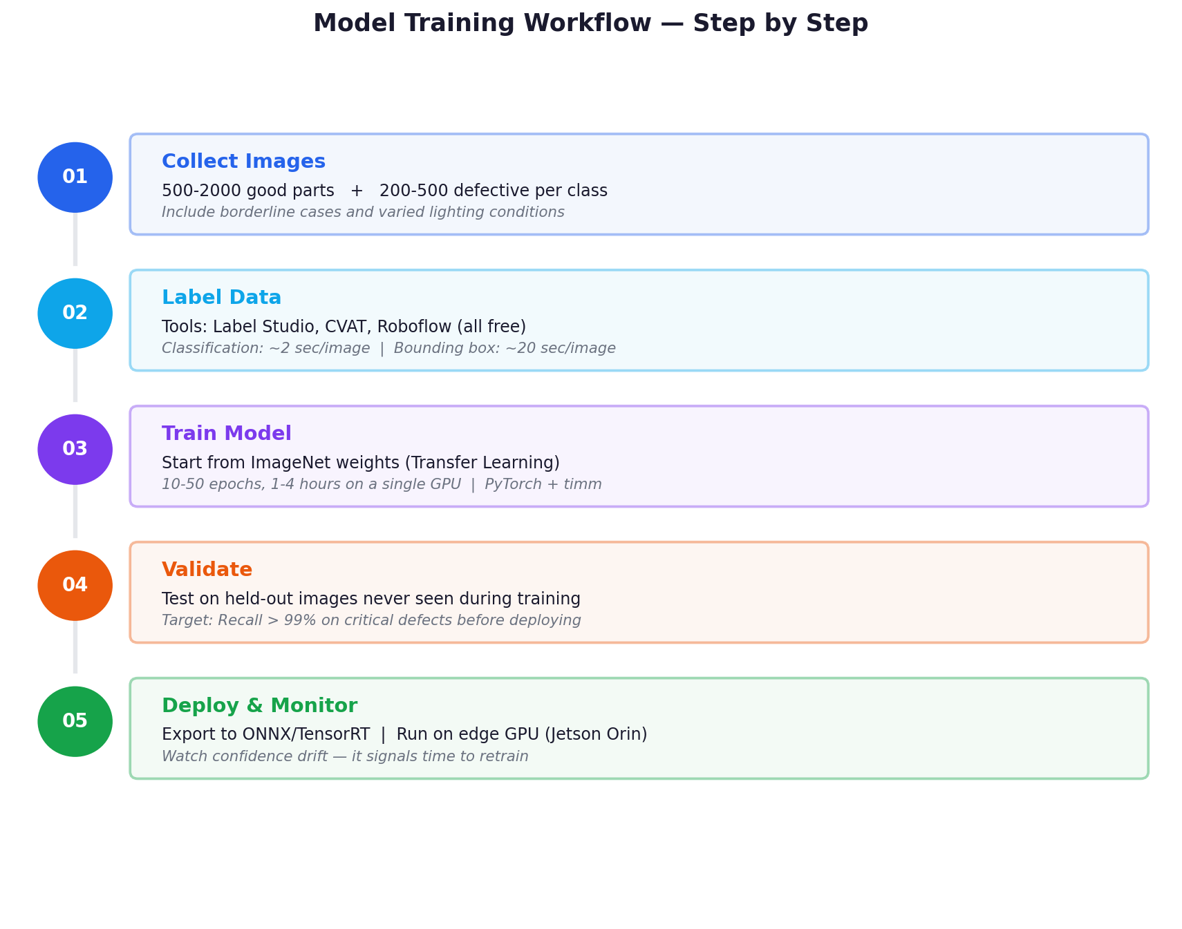
Step Details
Step 1: Collect Images Gather real production images, both good parts and defective ones. You need variety different lighting conditions, part orientations, defect severities. Aim for at least 500–2,000 images per class. Include borderline cases, where defects that are hard to call. These strengthen the model's decision boundary more than obvious defects do.
Step 2: Label Data Human experts annotate each image. For classification, assign a class label. For object detection, draw bounding boxes around defect locations. Free tools: Label Studio, CVAT, Roboflow. Budget ~2 seconds per classification image and ~20 seconds per bounding-box image.
Step 3: Train Model
Start from ImageNet weights (transfer learning). Fine-tune the top layers on your defect data. 10–50 training epochs, 1–4 hours on a single GPU. PyTorch with the timm library makes backbone selection a one-line change.
Step 4: Validate Test on held out images the model has never seen. Target: recall > 99% on critical defects before deploying. Tune your decision threshold to balance precision vs. recall based on the cost of each error type.
Step 5: Deploy and Monitor Export to ONNX or TensorRT format. Run inference on an edge GPU (NVIDIA Jetson Orin handles 200+ FPS at ~$500). Monitor confidence score distributions in production, a distribution shift signals that the real world has changed and the model needs retraining.
10. Evaluation Metrics
Understanding these four metrics is non-negotiable before deploying any defect detection system.

The most important tradeoff in manufacturing: A false negative (missed defect) is almost always more costly than a false positive (unnecessary rejection). Set your decision threshold accordingly, err on the side of higher recall, even if it means more false alarms to investigate.
11. Real-World Case Study
An automotive tier-1 supplier producing brake caliper castings needed to inspect weld integrity at 12 points per part. Line speed, 420 parts/hour. Previous approach: 2 human inspectors checking every 20th part.
System installed: 3× 5MP area-scan cameras, 1× structured light unit, YOLOv8-m fine-tuned on 3,200 labelled weld images, deployed on NVIDIA Jetson AGX Orin.
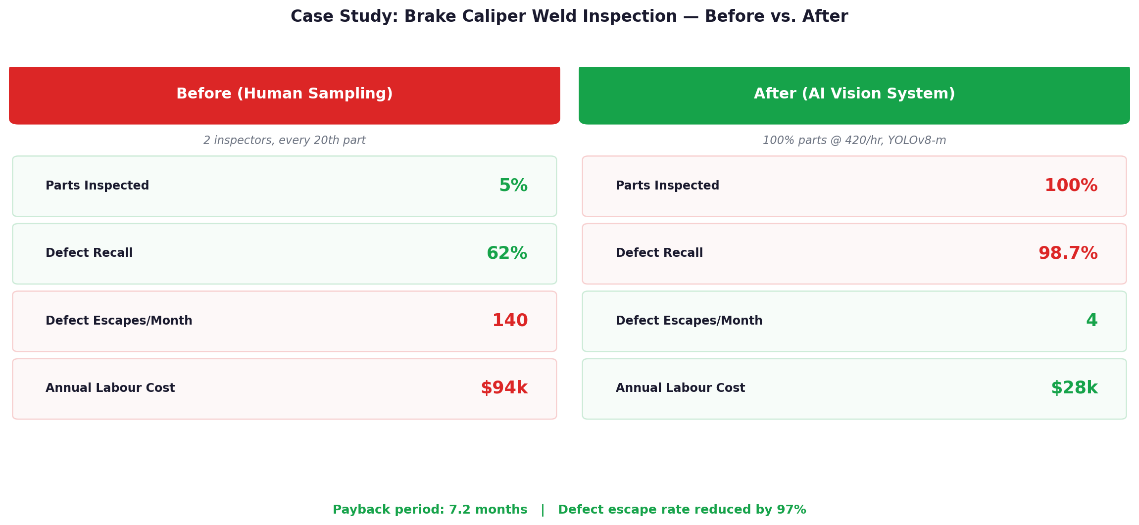
The model did not replace both inspectors. One moved to a quality engineer role managing the system and reviewing flagged images. The other transferred to a different line.
Why the 97% escape reduction? Not because the inspectors were failing, but because checking every single part is a fundamentally different statistical proposition than sampling 5%. At 5% sampling, a defect cluster during one shift can send hundreds of bad parts through before it's caught. At 100% coverage, nothing escapes.
12. What It Cannot Do Yet
Novel defect types If a defect type appears that was not in the training set, the model may misclassify or miss it. Monitor confidence score distributions in production. A shift signals time to retrain before escapes increase.
Data-scarce scenarios You need real examples to train on. If a defect appears fewer than ~50 times in production data, the model will underperform on it. Synthetic data generation (rendering defects onto clean-part images) helps, but does not fully substitute for real defect variation.
Lighting drift A model trained under one LED ring will degrade when that LED ages and dims by 15%. Consistent, monitored lighting is not optional. Some teams run a photometric calibration target at line start-up each shift to detect drift before it affects accuracy.
Internal or subsurface defects Camera-based vision sees surfaces only. Internal porosity, delamination, and sub-surface cracks require X-ray, CT scanning, or ultrasonic testing. AI-assisted readers exist for these too, but they are separate systems requiring different expertise.
Integration complexity The AI model is often the easiest part. Connecting it to PLCs, MES systems, rejection mechanisms, and operator alert workflows is where most projects hit friction. Budget 30–50% of total project time for integration, not modelling.
Summary
- Machine vision uses cameras and software to automate visual inspection on production lines
- AI vision uses CNNs (and increasingly Vision Transformers) trained on labelled defect images, no hand-coded rules needed
- The pipeline: Capture → Preprocess → Analyse → Classify → Act
- Good lighting matters as much as the model, it determines what defects are physically detectable at all
- CNNs learn local patterns (edges → textures → shapes → defect class); ViTs extend this with global self-attention across the entire image
- Transfer learning makes deployment practical with hundreds of images, not millions
- Optimise for recall, a missed defect almost always costs more than a false alarm
- Models drift when processes change — build retraining into your operations plan from day one
Comments (0)
No comments yet. Be the first to comment!